How Are Images REALLY Stored?

Intro

This post is me indulging in a rabbit hole. I somehow found myself thinking about images, probably after my recent exploration of some compression schemes. It’s common knowledge that images are either grayscale or RGB, that mixing red, green, and blue creates new colors. But there’s certainly more to storing an image than just aligning three-byte RGB values. Something about that idea piqued my curiosity, so this blog post is my attempt to scratch that itch and answer the question: how are images really stored?

Basics

An image is a collection of pixels. What is a pixel? It is the smallest unit of color in an image. Consider the following image from the famous MNIST dataset:

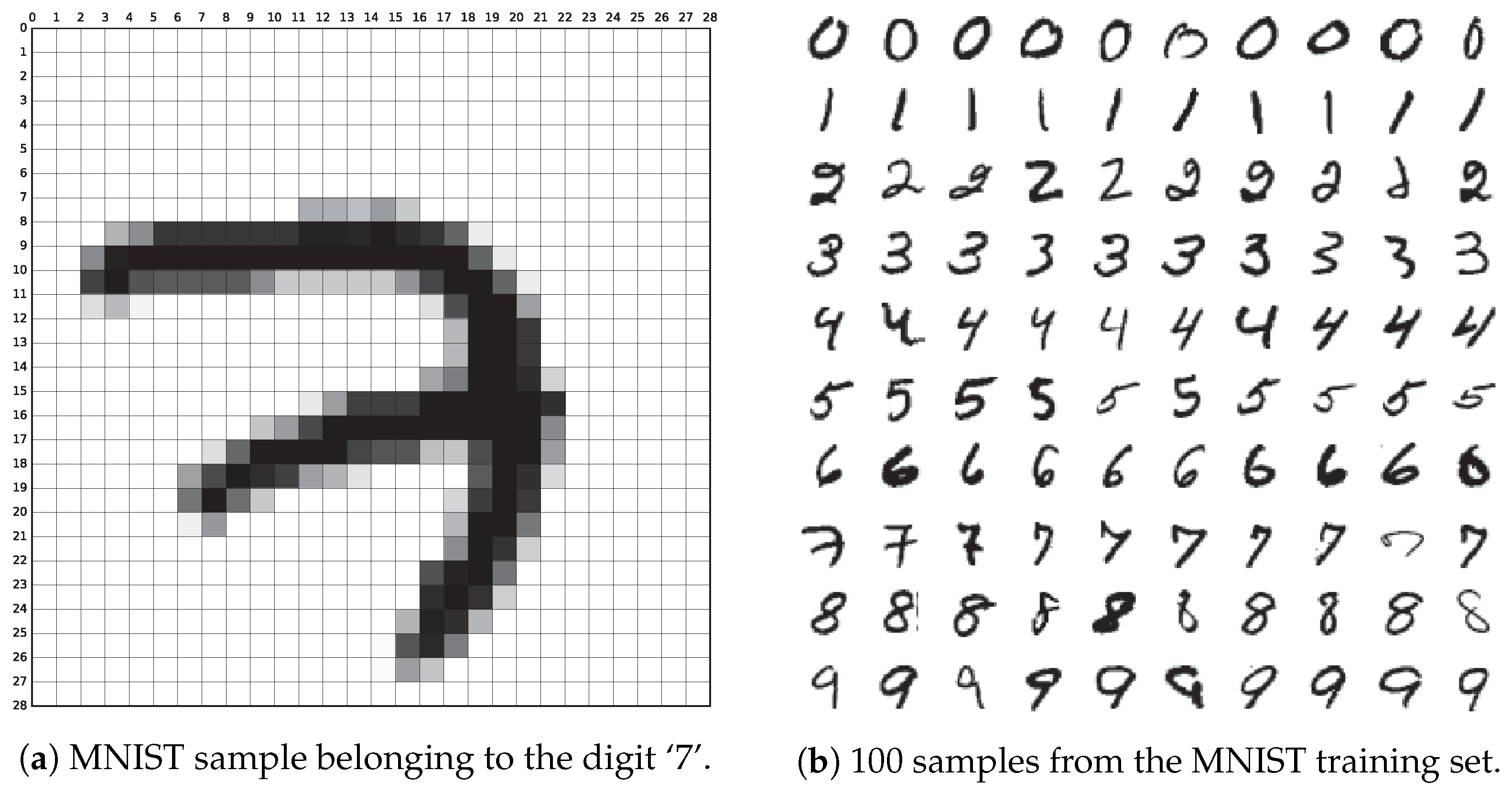
This image consists of 28x28 pixels (or squares). It is in grayscale, meaning each pixel has a value between 0 and 255, where 0 represents black and 255 represents white.

What about color images? Color images also use pixels, but each pixel is stored as an RGB triplet. For each pixel, 3 bytes represent its color: Red, Green, and Blue. (0, 0, 0) is black, and (255, 255, 255) is white. The idea is that with the absence of light (0, 0, 0), the color is black, and by mixing the maximum amount of each color, you get white. Red is (255, 0, 0), green is (0, 255, 0), and blue is (0, 0, 255).

RGB can have a fourth component called alpha, making it RGBA. Alpha indicates the opacity or transparency of a pixel. It is useful when composing images, as it dictates how transparency is handled. The more transparent a pixel is, the less it hides the background behind it. When two images are overlaid, the alpha value at each pixel determines the visibility of the background image through the corresponding pixel of the foreground image.

Consider the famous checkered pattern often used to indicate transparency. On the left side of the image, the opacity is high (alpha is high), making the background invisible. In contrast, on the right side, where the opacity is lower (alpha is low), the checkered background becomes visible.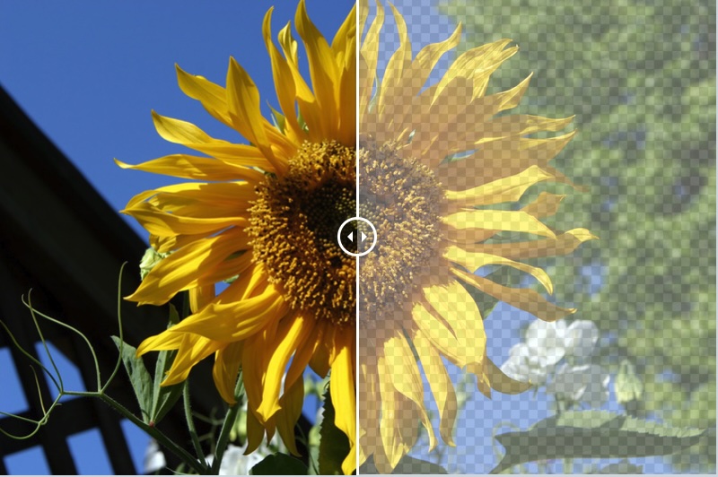

If we store a colored image (3 bytes per pixel) of size 1920x1080 uncompressed, we would need 1920x1080x3 = 6,220,800 bytes (about 6MB) for just one image!

1080p is common for videos today, while 240p (VHS resolution) is considered low-quality. 480p is ok-ish and corresponds to DVD quality.

If we were to stream uncompressed 1080p video at 24 frames per second, it would require more than 1 gigabit per second, which is enormous! So, unless there’s compression and other tricks, streaming high-quality video would be impossible.

Lossless compression algorithms typically achieve compression ratios of about 3:4 at best. The algorithms that achieve such high ratios are often compute-intensive and slow, making them unsuitable for real-time streaming. Even at a 3:4 ratio, it’s still not enough to stream high-resolution videos at high frame rates.

This is where lossy compression comes in. By discarding some data, we can achieve much better compression ratios. Lossy compression schemes often include a quality parameter, indicating how much quality we are willing to sacrifice in exchange for a better compression ratio.

Lossless Formats

GIF

Graphical Interchange Format, GIF (pronounced like “gif” from “gift”), is a lossless image compression format. It uses a fixed palette of 256 colors, each specified as 3 bytes for RGB. This means that instead of using 3 bytes to encode each pixel, we use an index pointing to one of the colors in the palette. The idea is that the palette colors offer enough nuance for the image. So, with 256 colors, we only need 1 byte for the index. This results in a compression ratio of 3:1. While it’s unlikely that the image in the real world has only 256 colors, some form of compression must have occurred before. However, GIF itself is not responsible for that compression.

Images are stored as a w × h array of 8-bit palette indices, which are then encoded using the famous LZ technique (backreferencing repeating sequences).
GIF is, of course, famous because it can store multiple images in a single file, which creates animated images.

Let’s take a look at the Golang standard library implementation of GIF. I think looking at how a list of images and the delays between them are used to produce a valid GIF should shed some light on the format:

images := []*image.Paletted{...}
// The successive delay times, one per frame, in 100ths of a second
// In this example, we have three images with 0.5 second delay between each
delays := []int{50,50,50} 
f, _ := os.OpenFile("amazing.gif", os.O_WRONLY|os.O_CREATE, 0600)
defer f.Close()
gif.EncodeAll(f, &gif.GIF{
    Image: images,
    Delay: delays, 
})

The API to create a GIF in Go is simple enough. Give a list of paletted images and the delay in between and save into our desired file.

Let’s take a look at Paletted:

package image

// Paletted is an in-memory image of uint8 indices into a given palette.
type Paletted struct {
	// Pix holds the image's pixels, as palette indices. The pixel at
	// (x, y) starts at Pix[(y-Rect.Min.Y)*Stride + (x-Rect.Min.X)*1].
	Pix []uint8
	// Stride is the Pix stride (in bytes) between vertically adjacent pixels.
	Stride int
	// Rect is the image's bounds.
	Rect Rectangle
	// Palette is the image's palette.
	Palette color.Palette
}

type Palette []Color

// Color can convert itself to alpha-premultiplied 16-bits per channel RGBA.
// The conversion may be lossy.
type Color interface {
	// RGBA returns the alpha-premultiplied red, green, blue and alpha values
	// for the color. Each value ranges within [0, 0xffff], but is represented
	// by a uint32 so that multiplying by a blend factor up to 0xffff will not
	// overflow.
	//
	// An alpha-premultiplied color component c has been scaled by alpha (a),
	// so has valid values 0 <= c <= a.
	RGBA() (r, g, b, a uint32)
}

// A Rectangle contains the points with Min.X <= X < Max.X, Min.Y <= Y < Max.Y.
// It is well-formed if Min.X <= Max.X and likewise for Y. Points are always
// well-formed. A rectangle's methods always return well-formed outputs for
// well-formed inputs.
type Rectangle struct {
	Min, Max Point
}

// A Point is an X, Y coordinate pair. The axes increase right and down.
type Point struct {
	X, Y int
}

A palette is defined by:

• A Rectangle, which is defined by its upper-left point (min) and lower-right point (max). Simple and effective! To make things simpler, let’s assume that Min = (0, 0).
• color.Palette, which is an array of Color interfaces, essentially serving as a holder for our RGB colors.
• Stride is the distance between two vertically adjacent pixels; it is often the row length, i.e., Max.X - Min.X.
• Pix is the actual data of the image. It is an index into the color palette. The array is one-dimensional but represents a 2D image. Let’s assume Min = (0, 0), The effective progression is as follows:
  • (0, 0), (1, 0), …, (Max.X-1, 0),
  • (0, 1), (1, 1), …, (Max.X-1, 1),
  • …,
  • (0, Max.Y-1), (1, Max.Y-1), …, (Max.X-1, Max.Y-1).

Simply, an image.Paletted is a list of colors and a list of pixels referencing those colors.

The paletted images and delays are used to initialize a GIF struct. Let’s inspect it:

// GIF represents the possibly multiple images stored in a GIF file.
type GIF struct {
	Image []*image.Paletted // The successive images.
	Delay []int             // The successive delay times, one per frame, in 100ths of a second.
	// LoopCount controls the number of times an animation will be
	// restarted during display.
	// A LoopCount of 0 means to loop forever.
	// A LoopCount of -1 means to show each frame only once.
	// Otherwise, the animation is looped LoopCount+1 times.
	LoopCount int
	// Disposal is the successive disposal methods, one per frame. For
	// backwards compatibility, a nil Disposal is valid to pass to EncodeAll,
	// and implies that each frame's disposal method is 0 (no disposal
	// specified).
	Disposal []byte
	// Config is the global color table (palette), width and height. A nil or
	// empty-color.Palette Config.ColorModel means that each frame has its own
	// color table and there is no global color table. Each frame's bounds must
	// be within the rectangle defined by the two points (0, 0) and
	// (Config.Width, Config.Height).
	//
	// For backwards compatibility, a zero-valued Config is valid to pass to
	// EncodeAll, and implies that the overall GIF's width and height equals
	// the first frame's bounds' Rectangle.Max point.
	Config image.Config
	// BackgroundIndex is the background index in the global color table, for
	// use with the DisposalBackground disposal method.
	BackgroundIndex byte
}

Let’s note that the number of loops is configurable and defaults to infinity when LoopCount == -1. We also observe that the GIF width and height are either configurable or inferred from the first image’s dimensions. This means that the GIF images can have different dimensions, and this is where we see the importance of Min and Max in each image’s rectangle: they need not be equal to the global Min and Max.

Disposal indicates how the previous frame should be disposed of. This parameter is directly linked to the alpha channel of RGBA, i.e., the transparency parameter. The main disposal methods are:

• Unspecified (Nothing): Replace one full-size, nontransparent frame with another.
• Do Not Dispose (Leave As Is): Any pixels not covered by the next frame continue to display.
• Restore to Background: Show the image specified in BackgroundIndex through the transparent pixels of the new frame.

Config can also hold a color.Palette, which is a global palette shared across all the images. Each image can have its own palette, or they can share one to save space if they are similar enough.

Ok. Now that we know what our structs look like, let’s dive into the actual encoding process:

// EncodeAll writes the images in g to w in GIF format with the
// given loop count and delay between frames.
func EncodeAll(w io.Writer, g *GIF) error {
	if len(g.Image) == 0 {
		return errors.New("gif: must provide at least one image")
	}
	if len(g.Image) != len(g.Delay) {
		return errors.New("gif: mismatched image and delay lengths")
	}
	e := encoder{g: *g}
    // ...

    
	if e.g.Config == (image.Config{}) {
        // If the image has no Config, we use the first image dimensions.
		p := g.Image[0].Bounds().Max
		e.g.Config.Width = p.X
		e.g.Config.Height = p.Y
	} else if e.g.Config.ColorModel != nil {
		if _, ok := e.g.Config.ColorModel.(color.Palette); !ok {
			return errors.New("gif: GIF color model must be a color.Palette")
		}
	}

    // ensure we have a proper write to send our data to
	if ww, ok := w.(writer); ok {
		e.w = ww
	} else {
		e.w = bufio.NewWriter(w)
	}

	e.writeHeader()
	for i, pm := range g.Image {
		disposal := uint8(0)
		if g.Disposal != nil {
			disposal = g.Disposal[i]
		}
		e.writeImageBlock(pm, g.Delay[i], disposal)
	}
	e.writeByte(sTrailer) // sTrailer = 0x3B => ascii semi-colon to signify EOF
	e.flush()
	return e.err
}

This function is refreshing. I love this kind of code. It reads like a normal paragraph. Check for errors, set the config, write the header then write each image block and finally write the EOF symbol and flush!

Here is writeHeader with some additional comment by yours truly:

func (e *encoder) writeHeader() {
	if e.err != nil {
		return
	}
	_, e.err = io.WriteString(e.w, "GIF89a") // Magic byte
	if e.err != nil {
		return
	}

	// Logical screen width and height.
	// written in Little Endian
	byteorder.LEPutUint16(e.buf[0:2], uint16(e.g.Config.Width))
	byteorder.LEPutUint16(e.buf[2:4], uint16(e.g.Config.Height))
	e.write(e.buf[:4])

    
	if p, ok := e.g.Config.ColorModel.(color.Palette); ok && len(p) > 0 {
		// write the global palette if we have it
		paddedSize := log2(len(p)) // Size of Global Color Table: 2^(1+n).
		e.buf[0] = fColorTable | uint8(paddedSize)
		e.buf[1] = e.g.BackgroundIndex
		e.buf[2] = 0x00 // Pixel Aspect Ratio.
		e.write(e.buf[:3])
		var err error
		e.globalCT, err = encodeColorTable(e.globalColorTable[:], p, paddedSize)
		if err != nil && e.err == nil {
			e.err = err
			return
		}
		e.write(e.globalColorTable[:e.globalCT])
	} else {
		// All frames have a local color table, so a global color table
		// is not needed.
		e.buf[0] = 0x00
		e.buf[1] = 0x00 // Background Color Index.
		e.buf[2] = 0x00 // Pixel Aspect Ratio.
		e.write(e.buf[:3])
	}

	// Add animation info if necessary.
	if len(e.g.Image) > 1 && e.g.LoopCount >= 0 {
		e.buf[0] = 0x21 // Extension Introducer.
		e.buf[1] = 0xff // Application Label.
		e.buf[2] = 0x0b // Block Size.
		e.write(e.buf[:3])
		_, err := io.WriteString(e.w, "NETSCAPE2.0") // Application Identifier.
		if err != nil && e.err == nil {
			e.err = err
			return
		}
		e.buf[0] = 0x03 // Block Size.
		e.buf[1] = 0x01 // Sub-block Index.
		byteorder.LEPutUint16(e.buf[2:4], uint16(e.g.LoopCount))
		e.buf[4] = 0x00 // Block Terminator.
		e.write(e.buf[:5])
	}
}

Here’s the loop that encodes the Palette table:

	for i, c := range p {
		if c == nil {
			return 0, errors.New("gif: cannot encode color table with nil entries")
		}
		var r, g, b uint8
		// It is most likely that the palette is full of color.RGBAs, so they
		// get a fast path.
		if rgba, ok := c.(color.RGBA); ok {
			r, g, b = rgba.R, rgba.G, rgba.B
		} else {
			rr, gg, bb, _ := c.RGBA()
			r, g, b = uint8(rr>>8), uint8(gg>>8), uint8(bb>>8)
		}
		dst[3*i+0] = r
		dst[3*i+1] = g
		dst[3*i+2] = b
	}

Nothing fancy. We loop over the colors and encode red,blue and green bytes consecutively in our destination buffer.

The actual image data is written in writeImageBlock. It is a tad long but the most interesting bit in my opinion is:

bw := blockWriter{e: e}
	bw.setup()
	lzww := lzw.NewWriter(bw, lzw.LSB, litWidth)
	if dx := rect.Dx(); dx == pm.Stride {
		_, e.err = lzww.Write(pm.Pix[:dx*rect.Dy()])
		if e.err != nil {
			lzww.Close()
			return
		}
	}

In the original code, rect is named b. I renamed it for clarity.
We take the Pix array of our image palette, where each value represents an index into the color array, then we compress it using the lzww scheme and write it down.

Voilà! That’s the magic behind GIF encoding.

I believe a decoder that displays the GIF image is where the true magic of the format lies, but this little exploration should give us a sense of what powers all those reaction memes that I personally use way too much.

Before moving on from GIF, let’s create a ridiculously simple GIF: 3 frames of blue, green, and red with a 1-second delay. Running go run main.go on this should generate an rgb.gif file that loops between the three colors.

package main

import (
	"fmt"
	"image"
	"image/color"
	"image/gif"
	"os"
)

func main() {
	var w, h int = 240, 240
	fileName := "rgb.gif"

	var palette = []color.Color{
		color.RGBA{0x00, 0x00, 0xff, 0xff}, // Blue
		color.RGBA{0x00, 0xff, 0x00, 0xff}, // Green
		color.RGBA{0xff, 0x00, 0x00, 0xff}, // Red
	}

	var images []*image.Paletted
	var delays []int
	for frame := 0; frame < len(palette); frame++ {
		img := image.NewPaletted(image.Rect(0, 0, w, h), palette)
		paletteIndex := uint8(frame) // paletteIndex 0 is blue, 1 is green and 2 is red
		for p := 0; p < 240*240; p++ {
			img.Pix[p] = paletteIndex
		}

		images = append(images, img)
		delays = append(delays, 100) // 1 second delay between frames
	}

	f, _ := os.OpenFile(fileName, os.O_WRONLY|os.O_CREATE, 0600)
	defer f.Close()
	gif.EncodeAll(f, &gif.GIF{
		Image: images,
		Delay: delays,
	})
	fmt.Printf("Created '%v'.\n", fileName)
}

PNG

Portable Network Graphic (PNG) was designed as successor to GIF. Unlike its precedessor, PNG supports non-paletted colors i.e. actually storing RGB or RGBA for each color. But it also supports grayscale and palettes with 3 bytes RGB or 4 bytes RGBA.

Every PNG file starts with the signature

89 50 4E 47 0D 0A 1A 0A

Then a list of chunks follows. There are different chunk types:

• IHDR (Image Header): This chunk must appear first and contains important image metadata like the width, height, bit depth, color type, etc.
• IDAT (Image Data): This chunk stores the actual image data, compressed using the Deflate algorithm (GZIP). The image data can be split across multiple IDAT chunks, especially for large images.
• IEND (End Chunk): This chunk marks the end of the PNG file.

I’m not a big fan of these abbreviation (IHDR, IDAT), they sound unnecessarily fancy to me.

Anyway, PNG uses the famous DEFLATE algorithm used by GZIP to compress the image data.

Filtering

The pixels are not always willing to be compressed. They can have a certain stubbornness. For instance, the pixel values can follow a pattern (2,4,6,8, etc). This pattern is unfortunately not amenable to LZ compression. We know that there is a repetitive behavior that governs the pixel values, but we can’t just use backreference.

The solution? Transform the problem set. Say we’ll subtract from each pixel its left neighbor. In our example, we’ll end up with (2,2,2,2, etc). This easily compressible. This technique is called a Sub Filter. Sometimes, there is a vertical pattern instead of a horizontal one e.g. pixel at line N are (12,18,44, 89) and just below them at line N+1, we have (13,19,45,90). This is not unlikely because often time we’ll have a gradient or graduation of colors. Here if we apply an Up Filter i.e. we subtract from each pixel its up neighbor, we end up with a neat (1,1,1,1), a perfect compression candidate.

PNG applies filters on a row basis. How do we pick a filter? There is no perfect way but the following heuristic is followed: minimize the sum of absolute differences between the original pixels and the filter pixels (up, before, etc). Why? Well, if the sum of the resulting differences (transformed pixels) is minimal, it is quite probable that we have a lot of close or similar values which are likely more compressible that distance values. I know one could come up with a compressible high distance example: (100, 100, 100, 100, 100, 100) whose sum is 600 is more compressible than (1,2,3,4,5,6) whose sum is way smaller. But it is a heuristic and my guess is that it has proven some nice empirical results. There are other techniques. libpng (the canonical implementation of PNG) has the following comment:

    * The prediction method we use is to find which method provides the
    * smallest value when summing the absolute values of the distances
    * from zero, using anything >= 128 as negative numbers.  This is known
    * as the "minimum sum of absolute differences" heuristic.  Other
    * heuristics are the "weighted minimum sum of absolute differences"
    * (experimental and can in theory improve compression), and the "zlib
    * predictive" method (not implemented yet), which does test compressions
    * of lines using different filter methods, and then chooses the
    * (series of) filter(s) that give minimum compressed data size (VERY
    * computationally expensive).
    *
    * GRR 980525:  consider also
    *
    *   (1) minimum sum of absolute differences from running average (i.e.,
    *       keep running sum of non-absolute differences & count of bytes)
    *       [track dispersion, too?  restart average if dispersion too large?]
    *
    *  (1b) minimum sum of absolute differences from sliding average, probably
    *       with window size <= deflate window (usually 32K)
    *
    *   (2) minimum sum of squared differences from zero or running average
    *       (i.e., ~ root-mean-square approach)
    */

The Golang implementation also uses the same heuristic as we shall see below.

Here is the list of all the filters PNG makes use of:

• None: Do nothing.
• Sub: Each byte is replaced by the difference between the current pixel and the previous one (on the same row).
• Up: Each byte is replaced by the difference between the current pixel and the pixel directly above it.
• Average: Each byte is replaced by the average of the pixel to the left and the pixel above.
• Paeth: Each byte is replaced by the difference between the current pixel and the best between the pixel to its left, above it, or upper-left.

Filter operations are done on a byte level and as result, in low-depth images (less than 8 bits per pixel), we default to the NONE filter.

Let’s get to brass tacks and look at the Go implementation of filters.

// Chooses the filter to use for encoding the current row, and applies it.
// The return value is the index of the filter and also of the row in cr that has had it applied.
func filter(cr *[nFilter][]byte, pr []byte, bpp int) int {
	// We try all five filter types, and pick the one that minimizes the sum of absolute differences.
	// This is the same heuristic that libpng uses, although the filters are attempted in order of
	// estimated most likely to be minimal (ftUp, ftPaeth, ftNone, ftSub, ftAverage), rather than
	// in their enumeration order (ftNone, ftSub, ftUp, ftAverage, ftPaeth).
	cdat0 := cr[0][1:]
	cdat1 := cr[1][1:]
	cdat2 := cr[2][1:]
	cdat3 := cr[3][1:]
	cdat4 := cr[4][1:]
	pdat := pr[1:]
	n := len(cdat0)

	// The up filter.
	sum := 0
	for i := 0; i < n; i++ {
		cdat2[i] = cdat0[i] - pdat[i]
		sum += abs8(cdat2[i])
	}
	best := sum
	filter := ftUp

	// The Paeth filter.
	sum = 0
	for i := 0; i < bpp; i++ {
		cdat4[i] = cdat0[i] - pdat[i]
		sum += abs8(cdat4[i])
	}
	for i := bpp; i < n; i++ {
		cdat4[i] = cdat0[i] - paeth(cdat0[i-bpp], pdat[i], pdat[i-bpp])
		sum += abs8(cdat4[i])
		if sum >= best {
			break
		}
	}
	if sum < best {
		best = sum
		filter = ftPaeth
	}

	// The none filter.
	sum = 0
	for i := 0; i < n; i++ {
		sum += abs8(cdat0[i])
		if sum >= best {
			break
		}
	}
	if sum < best {
		best = sum
		filter = ftNone
	}

	// The sub filter.
	sum = 0
	for i := 0; i < bpp; i++ {
		cdat1[i] = cdat0[i]
		sum += abs8(cdat1[i])
	}
	for i := bpp; i < n; i++ {
		cdat1[i] = cdat0[i] - cdat0[i-bpp]
		sum += abs8(cdat1[i])
		if sum >= best {
			break
		}
	}
	if sum < best {
		best = sum
		filter = ftSub
	}

	// The average filter.
	sum = 0
	for i := 0; i < bpp; i++ {
		cdat3[i] = cdat0[i] - pdat[i]/2
		sum += abs8(cdat3[i])
	}
	for i := bpp; i < n; i++ {
		cdat3[i] = cdat0[i] - uint8((int(cdat0[i-bpp])+int(pdat[i]))/2)
		sum += abs8(cdat3[i])
		if sum >= best {
			break
		}
	}
	if sum < best {
		filter = ftAverage
	}

	return filter
}

The function takes in cr *[nFilter][]byte, pr []byte, bpp int. cr is an array of arrays (I’ll use array and slice interchangeably), it represents the current row for which we want to pick a filter (the return value is the filter index/type).

Each filter result is calculated within the cr[filterNb] slice (array). As the comment says, the filters are tested in the order of most likely to be minimal, this is to be able to break early in subsequent filter as soon as the sum of diffs exceeds the current best. pr is the previous row. The first byte of each row’s byte array contains the filter type this is why pdat = pr[1:], it is the previous row’s data without the filter type. Let’s dissect the up filter.

	// The up filter.
	sum := 0
	for i := 0; i < n; i++ { // loop over the row pixels
		cdat2[i] = cdat0[i] - pdat[i] // subsctract the previous row's pixel at the same position i.e. the pixel above
		sum += abs8(cdat2[i]) // add the absolute difference to our sum which we are trying to minimize
	}

How about the sub filter?

	// The sub filter.
	// bpp is bytes per pixel. For RGB, it's 3. For gray scale, it's 1.
	sum = 0
	for i := 0; i < bpp; i++ {
		cdat1[i] = cdat0[i]
		sum += abs8(cdat1[i])
	}
	for i := bpp; i < n; i++ {
		cdat1[i] = cdat0[i] - cdat0[i-bpp] // subtract each byte within a pixel from corresponding byte in previous pixel
		sum += abs8(cdat1[i])
		if sum >= best { // break early if this is worse than previous filter
			break
		}
	}

bpp plays a crucial role here. Notice how in the subtraction cdat1[i] = cdat0[i] - cdat0[i - bpp], we are subtracting the pixel bpp positions before the current pixel. In the case of RGB, this means we subtract the previous pixel’s red value from the current pixel’s red, the previous green from the current green, and so on.

We calculate the sum for each filter and take the min which represents our chosen filter supposed to maximize our DEFLATE compression and that’s it. The result of the chosen filter will be available in the cr[chosenFilter] array.

Encoding

Let’s take a look at the Encode method used to encode PNG images.

// Encode writes the Image m to w in PNG format.
func (enc *Encoder) Encode(w io.Writer, m image.Image) error {
	// Obviously, negative widths and heights are invalid. Furthermore, the PNG
	// spec section 11.2.2 says that zero is invalid. Excessively large images are
	// also rejected.
	mw, mh := int64(m.Bounds().Dx()), int64(m.Bounds().Dy())
	if mw <= 0 || mh <= 0 || mw >= 1<<32 || mh >= 1<<32 {
		return FormatError("invalid image size: " + strconv.FormatInt(mw, 10) + "x" + strconv.FormatInt(mh, 10))
	}

	e := &encoder{}
	//....

	e.enc = enc
	e.w = w
	e.m = m

	var pal color.Palette
	// cbP8 encoding needs PalettedImage's ColorIndexAt method.
	if _, ok := m.(image.PalettedImage); ok {
		pal, _ = m.ColorModel().(color.Palette)
	}
	if pal != nil {
		if len(pal) <= 2 {
			e.cb = cbP1
		} else if len(pal) <= 4 {
			e.cb = cbP2
		} else if len(pal) <= 16 {
			e.cb = cbP4
		} else {
			e.cb = cbP8
		}
	} else {
		switch m.ColorModel() {
		case color.GrayModel:
			e.cb = cbG8
		case color.Gray16Model:
			e.cb = cbG16
		case color.RGBAModel, color.NRGBAModel, color.AlphaModel:
			if opaque(m) {
				e.cb = cbTC8
			} else {
				e.cb = cbTCA8
			}
		default:
			if opaque(m) {
				e.cb = cbTC16
			} else {
				e.cb = cbTCA16
			}
		}
	}

	_, e.err = io.WriteString(w, pngHeader)
	e.writeIHDR()
	if pal != nil {
		e.writePLTEAndTRNS(pal)
	}
	e.writeIDATs()
	e.writeIEND()
	return e.err
}

A lot to unpack. Fun! First of all comments like Obviously, negative widths and heights are invalid are one of the reason I love to read code. It just sounds nice.

We start by checking that our images dimensions make then we init our encoder which is defined as (I added the comments):

type encoder struct {
	enc     *Encoder
	w       io.Writer
	m       image.Image
	cb      int //  a combination of color type and bit depth.
	err     error
	header  [8]byte
	footer  [4]byte
	tmp     [4 * 256]byte
	cr      [nFilter][]uint8 // stores the current row and possible filter
	pr      []uint8          // previous row
	zw      *zlib.Writer     // used of compression
	zwLevel int              // compression level
	bw      *bufio.Writer
}

Afterwards, we try to cast our image into a image.PalettedImage then we try to extract the a Palette (which is an alias for []Color). If we succeed, this means our image is paletted and we assign the depth (number of bits) based on the number of colors in the palette. Otherwise, based on the returned type of ColorModel, we assign our cb. GrayModel, Gray16Model, RGBAModel, AlphaModel are exactly what their name says.

Once we know the color type and depth, the remaining code is almost plain english

	_, e.err = io.WriteString(w, pngHeader) // write magic "\x89PNG\r\n\x1a\n"
	e.writeIHDR() // write the actual header 
	if pal != nil {
		e.writePLTEAndTRNS(pal) // write the palette, if there is one
	}
	e.writeIDATs() // the image data
	e.writeIEND() // write the footer: `IEND`

Here is writeIHDR preceded by the color types:

// Color type, as per the PNG spec.
const (
	ctGrayscale      = 0
	ctTrueColor      = 2
	ctPaletted       = 3
	ctGrayscaleAlpha = 4
	ctTrueColorAlpha = 6
)

func (e *encoder) writeIHDR() {
	b := e.m.Bounds()
	// Write image dimensions in BigEndian (most significant byte at the smallest memory address)
	binary.BigEndian.PutUint32(e.tmp[0:4], uint32(b.Dx())) // image width
	binary.BigEndian.PutUint32(e.tmp[4:8], uint32(b.Dy())) // image height
	// Set bit depth and color type.
	switch e.cb {
	case cbG8:
		e.tmp[8] = 8
		e.tmp[9] = ctGrayscale
	case cbTC8:
		e.tmp[8] = 8
		e.tmp[9] = ctTrueColor
	case cbP8:
		e.tmp[8] = 8
		e.tmp[9] = ctPaletted
	case cbP4:
		e.tmp[8] = 4
		e.tmp[9] = ctPaletted
	case cbP2:
		e.tmp[8] = 2
		e.tmp[9] = ctPaletted
	case cbP1:
		e.tmp[8] = 1 // 1 bit per Pixel !!!!
		e.tmp[9] = ctPaletted
	case cbTCA8:
		e.tmp[8] = 8
		e.tmp[9] = ctTrueColorAlpha
	case cbG16:
		e.tmp[8] = 16
		e.tmp[9] = ctGrayscale
	case cbTC16:
		e.tmp[8] = 16
		e.tmp[9] = ctTrueColor
	case cbTCA16:
		e.tmp[8] = 16
		e.tmp[9] = ctTrueColorAlpha
	}
	e.tmp[10] = 0 // default compression method
	e.tmp[11] = 0 // default filter method
	e.tmp[12] = 0 // non-interlaced
	e.writeChunk(e.tmp[:13], "IHDR")
}

We prepare our 13 bytes array header and write it as the IHDR chunk using writeChunk

func (e *encoder) writeChunk(b []byte, name string) {
	if e.err != nil {
		return
	}
	// 4 Gib max chunk size
	n := uint32(len(b))
	if int(n) != len(b) {
		e.err = UnsupportedError(name + " chunk is too large: " + strconv.Itoa(len(b)))
		return
	}
	// add the chunk length
	binary.BigEndian.PutUint32(e.header[:4], n)
	// chunk name
	e.header[4] = name[0]
	e.header[5] = name[1]
	e.header[6] = name[2]
	e.header[7] = name[3]
	crc := crc32.NewIEEE()
	// CRC check for the name + actual chunk data
	crc.Write(e.header[4:8])
	crc.Write(b)
	binary.BigEndian.PutUint32(e.footer[:4], crc.Sum32())

	// write header (length + name)
	_, e.err = e.w.Write(e.header[:8])
	if e.err != nil {
		return
	}
	// actual data
	_, e.err = e.w.Write(b)
	if e.err != nil {
		return
	}
	// CRC
	_, e.err = e.w.Write(e.footer[:4])
}

I added comments, but the code is fairly simple. It writes the length and chunk name, then the actual bytes, and finally adds the CRC.

If our color scheme has a palette, we write a PLTE chumk using:

func (e *encoder) writePLTEAndTRNS(p color.Palette) {
	if len(p) < 1 || len(p) > 256 {
		e.err = FormatError("bad palette length: " + strconv.Itoa(len(p)))
		return
	}
	last := -1
	for i, c := range p {
		c1 := color.NRGBAModel.Convert(c).(color.NRGBA)
		e.tmp[3*i+0] = c1.R
		e.tmp[3*i+1] = c1.G
		e.tmp[3*i+2] = c1.B
		if c1.A != 0xff {
			last = i
		}
		e.tmp[3*256+i] = c1.A
	}
	e.writeChunk(e.tmp[:3*len(p)], "PLTE")
	if last != -1 {
		e.writeChunk(e.tmp[3*256:3*256+1+last], "tRNS")
	}
}

The PLTE chunk always stores palette colors using 3 bytes, regardless of the color type, meaning even grayscale colors (1 byte) use 3 bytes. The tRNS chunk stores transparency information, with the alpha byte for each color palette placed after the palette color bytes.

Finally, the meat and potatoes are the actual image data, written using writeIDATs:

// Write the actual image data to one or more IDAT chunks.
func (e *encoder) writeIDATs() {
	if e.err != nil {
		return
	}
	if e.bw == nil {
		e.bw = bufio.NewWriterSize(e, 1<<15)
	} else {
		e.bw.Reset(e)
	}
	e.err = e.writeImage(e.bw, e.m, e.cb, levelToZlib(e.enc.CompressionLevel))
	if e.err != nil {
		return
	}
	e.err = e.bw.Flush()
}

Its core is this loop within writeImage:

	for y := b.Min.Y; y < b.Max.Y; y++ {
		// Convert from colors to bytes.
		i := 1
		switch cb {
		case cbG8:
			if gray != nil {
				offset := (y - b.Min.Y) * gray.Stride
				copy(cr[0][1:], gray.Pix[offset:offset+b.Dx()])
			} else {
				for x := b.Min.X; x < b.Max.X; x++ {
					c := color.GrayModel.Convert(m.At(x, y)).(color.Gray)
					cr[0][i] = c.Y
					i++
				}
			}
		// omitted ...
		case cbTC8:
			// We have previously verified that the alpha value is fully opaque.

			// omitted ...
				for x := b.Min.X; x < b.Max.X; x++ {
					r, g, b, _ := m.At(x, y).RGBA()
					cr0[i+0] = uint8(r >> 8)
					cr0[i+1] = uint8(g >> 8)
					cr0[i+2] = uint8(b >> 8)
					i += 3
				}
		
		case cbP8:
			// omitted ...
				pi := m.(image.PalettedImage)
				for x := b.Min.X; x < b.Max.X; x++ {
					cr[0][i] = pi.ColorIndexAt(x, y)
					i += 1
				}

		// omitted ...
		}

		// Apply the filter.
		// Skip filter for NoCompression and paletted images (cbP8) as
		// "filters are rarely useful on palette images" and will result
		// in larger files (see http://www.libpng.org/pub/png/book/chapter09.html).
		f := ftNone
		if level != zlib.NoCompression && cb != cbP8 && cb != cbP4 && cb != cbP2 && cb != cbP1 {
			// Since we skip paletted images we don't have to worry about
			// bitsPerPixel not being a multiple of 8
			bpp := bitsPerPixel / 8
			f = filter(&cr, pr, bpp)
		}

		// Write the compressed bytes.
		if _, err := e.zw.Write(cr[f]); err != nil {
			return err
		}

		// The current row for y is the previous row for y+1.
		pr, cr[0] = cr[0], pr
	}

I kept only the grayscale, RGB (true color), and 256-color palette cbP8 cases. As you can see, we loop over the rows of our images: y := b.Min.Y; y < b.Max.Y; y++. For each row, if it is grayscale (cbG8), we copy 1 byte for each color. If it is RGB, we copy 3 bytes. For the paletted case, we just write the palette index.

Afterwards, if compression is enabled (level != zlib.NoCompression)—there’s no need to filter if we won’t compress—and we are not using palettes, we choose a filter for our image data using the filter function we explored earlier. Then, we pass our filtered (or unfiltered) bytes to the LZ writer, and our compressed image data is ready to be flushed.

Finally, we add our last chunk using writeIEND, which is short and sweet:

func (e *encoder) writeIEND() { e.writeChunk(nil, "IEND") }

And that’s the gist of PNG!

Lossy Images

JPEG

JPEG, Joint Photographic Experts Group (what a name, by the way!), is extremely prevalent across the web. Anybody who played with images on a computer has probably interacted with either PNG or JPEG. It can achieve high compression ratios, reducing the original image by up to +90% of its size while keeping an acceptable quality. The compression ratio ranges from 5:1 to 50:1. The quality is tunable, and we can trade off compression ratio for better quality.

JPEG is a magical feat of engineering and consists of multiple steps. Let’s try to explore some of its fundamental ideas and look at some code. Coming up: chroma subsampling, DCT (Discrete Cosine Transform), and quantization.

YCbCr and Chroma Subsumpling

This step is based on the following idea: the human eye is more sensitive to brightness (luma) and green than it is to red and blue (chroma).

If we transform our RGB color to an equivalent that isolates luminance from the red and blue components, we can retain the luma bits (which our eyes are most sensitive to) while compressing (subsampling) the chroma (red and blue), which we are less sensitive to.

Well, such a transformation exists and is called YCbCr (Y: Luma, Cb: Chroma Blue, Cr: Chroma Red), which separates brightness (Y) from the color information (Cb and Cr).

Given that our eyes are more sensitive to brightness than colors, we can compress our original image by sampling less of the CbCr components and keeping all of the luma components. This is called chroma subsampling, i.e., we take less information from the colors/chroma. For each set of 4 pixels, we subsample them by replacing them with one pixel (such as averaging or taking the top-left pixel). By replacing 4 pixels with 1 for both Cb and Cr, we shrink the original size by 50%.

JPEG works on 8x8 pixel blocks. Here is the function the Go standard library uses to convert to YCbCr:

const blockSize = 64
type block [blockSize]int32 // block holds 64 (8x8) pixels

// toYCbCr converts the 8x8 region of m whose top-left corner is p to its
// YCbCr values.
func toYCbCr(m image.Image, p image.Point, yBlock, cbBlock, crBlock *block) {
	b := m.Bounds()
	xmax := b.Max.X - 1
	ymax := b.Max.Y - 1
	for j := 0; j < 8; j++ { // 8x8 pixel blocks
		for i := 0; i < 8; i++ {
			r, g, b, _ := m.At(min(p.X+i, xmax), min(p.Y+j, ymax)).RGBA()
			yy, cb, cr := color.RGBToYCbCr(uint8(r>>8), uint8(g>>8), uint8(b>>8))
			yBlock[8*j+i] = int32(yy)
			cbBlock[8*j+i] = int32(cb)
			crBlock[8*j+i] = int32(cr)
		}
	}
}

The magic conversion really happens within RGBToYCbCr:

// RGBToYCbCr converts an RGB triple to a Y'CbCr triple.
func RGBToYCbCr(r, g, b uint8) (uint8, uint8, uint8) {
	// The JFIF specification says:
	//	Y' =  0.2990*R + 0.5870*G + 0.1140*B
	//	Cb = -0.1687*R - 0.3313*G + 0.5000*B + 128
	//	Cr =  0.5000*R - 0.4187*G - 0.0813*B + 128
	// https://www.w3.org/Graphics/JPEG/jfif3.pdf says Y but means Y'.

	yy := (19595*r1 + 38470*g1 + 7471*b1 + 1<<15) >> 16
	// omitted ...
	cb := -11056*r1 - 21712*g1 + 32768*b1 + 257<<15
	// omitted ...
	cr := 32768*r1 - 27440*g1 - 5328*b1 + 257<<15
	// omitted ...
	return uint8(yy), uint8(cb), uint8(cr)
}

It is simply a linear conversion. We notice that Y is mostly green but also has some red and blue in it. As we said, this is luma, and our eye is most sensitive to it; this represents the brightness of the image. Cb and Cr can be interpreted as color differences for blue and red from the luminance.

This tremendous lecture (I love the whole lecture series, and the professor is just a delight to follow) shows a great deal of examples and how tweaking different values from RGB and YCbCr can impact the resulting image. It is quite uncanny how reducing the depth (fewer bits/info) for Cb and Cr has much less effect than reducing blue or red in an RGB space.
This is neuroscience meets engineering.
One interesting insight from this is how optimized the world is for human biology. This is similar to how glasses are made for the human face, ears, and eyes. It also makes me think that robots are best made humanoid to be most effective since our world is engineered for us.

Ok, enough philosophizing, how is the chroma subsampling actually done?

Here is the loop that writes the image data in JPEG:

	cb, cr [4]block
	// omitted
	for y := bounds.Min.Y; y < bounds.Max.Y; y += 16 {
			for x := bounds.Min.X; x < bounds.Max.X; x += 16 {
				for i := 0; i < 4; i++ {
					xOff := (i & 1) * 8
					yOff := (i & 2) * 4
					p := image.Pt(x+xOff, y+yOff)
					// omitted ..
					toYCbCr(m, p, &b, &cb[i], &cr[i])
					prevDCY = e.writeBlock(&b, 0, prevDCY)
				}
				scale(&b, &cb)
				prevDCCb = e.writeBlock(&b, 1, prevDCCb)
				scale(&b, &cr)
				prevDCCr = e.writeBlock(&b, 1, prevDCCr)
			}
		}

cb and cr each hold 4 blocks of 8x8 Cb and Cr pixels. We are looping over a 16x16 region from the original image, which consists of 4 8x8 blocks. These are placed in the cb and cr variables.

The innermost loop has a rather cool trick. Notice xOff := (i & 1) * 8 and yOff := (i & 2) * 4. Their values for i = [0,1,2,3] are (xOff, yOff) = [(0,0), (8,0), (0,8), (8,8)]. This advances within the 16x16 block from the top left, then shifts to the right by 8 (next 8x8 block to the right), and then moves to the next line to do the same thing.

So we have our Cb and Cr values in 4 8x8 blocks. The subsampling happens in scale:

// scale scales the 16x16 region represented by the 4 src blocks to the 8x8
// dst block.
func scale(dst *block, src *[4]block) {
	for i := 0; i < 4; i++ {
		dstOff := (i&2)<<4 | (i&1)<<2
		for y := 0; y < 4; y++ {
			for x := 0; x < 4; x++ {
				j := 16*y + 2*x
				sum := src[i][j] + src[i][j+1] + src[i][j+8] + src[i][j+9]
				dst[8*y+x+dstOff] = (sum + 2) >> 2
			}
		}
	}
}

This is something! First, notice that we are taking a [4]block src and transforming it into a block dst. Remember that block is just an array of size 64 (8x8).

i represents the top left, top right, bottom left, and bottom right 8x8 blocks within the 16x16 input region. Each one of the 8x8 blocks will map to a 4x4 block (1/4 shrinkage). Each pixel of the 4x4 block is represented by x and y. How does each pixel get its value?

j := 16*y + 2*x // top left point of the 4 pixel square
sum := src[i][j] + src[i][j+1] + src[i][j+8] + src[i][j+9] // sum of pixel square values starting at j
dst[8*y+x+dstOff] = (sum + 2) >> 2 // divide by 4 (>>2) to get the average but add 2 before to round up instead of down

This is simply averaging the 4 pixel values using a 2-bit right shift and making sure we are rounding up by adding 2 before that.

The value of dstOff is intriguing. For i=[0,1,2,3], we get dstOff=[0,4,32,36]. What do these values mean?

Let’s remember that each i represents a 4x4 block within our target 8x8 block, which represents our scaled-down 16x16. If we visualize an 8x8 matrix, the top-left block starts at (0,0). The top-right block starts at (4,0). The bottom-left block starts at (4,0), and the bottom-right block starts at (4,4). If we translate those into a 1D representation using x + 8y, we get:

0 + 0 * 8 = 0 
4 + 0 * 8 = 4
0 + 4 * 8 = 32
4 + 4 * 8 = 36

Which represents the start of each 4x4 block. This calculation is done in a fancy way with dstOff := (i&2)<<4 | (i&1)<<2.
(i&2)<<4 will be 32 for values that have the second bit set to one, i.e., 2 (10) and 3 (11) (second row), and (i&1)<<2 will be 4 for values 1 (01) and 3 (11). Binary magic at its finest!

If you’re wondering why go through all this trouble and have 4 blocks from a 16x16 region instead of treating them separately, the reason is that we want to end up with an 8x8 block similar to the Y (luma) component. This ensures that the next JPEG step, namely the Discrete Cosine Transform (DCT), operates on the same dimensions.

To sum up, the scale function is simply averaging 4 pixels into 1, thus scaling down 4 8x8 blocks into a single one.

Direct Cosine Transform

So, we achieved a healthy 50% shrinkage using YCbCr. However, we’re still far from unlocking JPEG’s full potential.

The next step in the process is the Discrete Cosine Transform (DCT). In short, DCT isolates and identifies parts of an image that can be trimmed or discarded without significantly affecting its quality.

We can think of an image as a function. Each pixel in the image corresponds to a position (x, y) with a value indicating its color intensity. We could represent this as F(x, y) = pixelValue. If we agree to traverse the image from left to right and top to bottom, we can simplify things by using a single variable x', where x' = x + len(row) * y (this is essentially what the Golang implementation does with its 64-bit unsigned integer blocks).

In other words, an image is a function. So what? one might ask. Well, what if there was a way to approximate this function with various components of varying importance and save space by discarding least important ones.

Imagine we had a set of tuples like (1, 2), (2, 4), ..., (10, 20), (1000, 2000). We could store 2 * 1000 numbers, or we could realize that this relationship follows a simple pattern: f(x) = 2x. Instead of storing all the points, we could store just the formula, yielding significant space savings.

DCT allows us to represent an image function as a sum of well-known cosine functions of increasing frequency. This is mathematically proven to be feasible.

What’s truly remarkable about this representation is that the human eye (biology strikes again) is less sensitive to high-frequency details than to lower-frequency ones. Even more interesting, high-frequency components represent rapid changes in the image, and in general, images are dominated by low-frequency components. In other words, colors in images don’t typically change abruptly.

To put it another way, any 8x8 pixel block can be expressed as a weighted sum of the following 64 blocks:

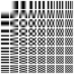
Let’s think about that again. Any 8x8 block can be expressed as a combination of these 64 blocks. And the more we approach to bottom right the higher frequencies get and the less our eyes can really discern.

So if we represent our 8x8 block with only a few weights of these lower frequency DCT blocks - say with just 16 or 32 weights (instead of 64 pixel), we would achieve great savings and not degrade the quality.

To prevent my Mathjax plugin from accumulating too much dust and give my rambling some cachet, let’s look at the actual formula:

\[X_{k}=\sum _{n=0}^{N-1}x_{n}\cos \left[\,{\tfrac {\,\pi \,}{N}}\left(n+{\tfrac {1}{2}}\right)k\,\right]\qquad {\text{ for }}~k=0,\ \dots \ N-1~\]

This is how we calculate the coefficient of the Kth cosine function.

A helpful way to think about this equation is that it calculates the dot product between our N pixel values \(x_{n}\) and N samples from a cosine function: \(\cos \left[\,{\tfrac {\,\pi \,}{N}}\left(n+{\tfrac {1}{2}}\right)k\,\right]\) whose frequency increases with k.

The coefficient represents the degree of similarity (i.e., the dot product) between our pixel values and the cosine function.

For our purposes, we are working with one of the 64 blocks (note that the above cosine function is 1-D, while the block is 2-D, so this applies to just one dimension of the block).

For example, if we had an 8x8 grid of input pixels that perfectly matches one of the cosine blocks, the computed coefficient for that block would be 1, and the coefficients for the other blocks would be 0. This is because that particular block alone is sufficient to represent the input.

One more time: a weighted combination of low-frequency blocks (closer to the top-left) is more likely to represent the input 8x8 pixel blocks. So, when we express our input as 64 coefficients of blocks, we can truncate or discard the high-frequency ones.

Ok, we are now ready for the 2D formula:

\[X_{k,l} = \sum_{n=0}^{N-1} \sum_{m=0}^{N-1} x_{n,m} \cos\left[\frac{\pi}{N} \left(n + \frac{1}{2}\right) k \right] \cos\left[\frac{\pi}{N} \left(m + \frac{1}{2}\right) l \right]\]

And translated to code, we get the following:

    for i := 0; i < N; i++ {
        for j := 0; j < N; j++ {
            temp := 0.0
            for x := 0; x < N; x++ {
                for y := 0; y < N; y++ {
                    temp += Cosines[x][i] * Cosines[y][j] * Pixel[x][y]
                }
            }
            temp *= math.Sqrt(2 * float64(N)) * Coefficient[i][j]
            DCT[i][j] = int(math.Round(temp))
        }
    }

The cosines array already holds the precomputed values. We iterate over the pixels and calculate the output coefficients, which depend on the pixel values and the cosines.

However, as one can see, a nesting level of 4 is not far from desirable. Practical implementations use an optimized version known as the Fast DCT, which is more computationally efficient.

Quantization

Instead of deleting high coefficients outright, we reduce their precision by using fewer bits to store them. This process is called quantization. As a result, the important low coefficients are stored with higher fidelity, while the high coefficients are quantized to save space.

How is this done in practice?

DCT output is deivided by a Q table, reducing the number of bits. For example, if the DCT output is 31 and Q is 2, Round(31/Q) gives 16. If Q is 4, Round(31/Q) gives 8. To recover the original values, we multiply the quantized result by Q, though the recovered value will be an approximation.

The JPEG standard provides a table to quantize each of the 64 coefficients resulting from applying the DCT to an 8x8 pixel block.

Since chroma components (Yb and Yr) have less impact on our perception, their quantization tables are more aggressive than the one used for luma (Y). Here are the tables:

var unscaledQuant = [nQuantIndex][blockSize]byte{
	// Luminance.
	{
		16, 11, 12, 14, 12, 10, 16, 14,
		13, 14, 18, 17, 16, 19, 24, 40,
		26, 24, 22, 22, 24, 49, 35, 37,
		29, 40, 58, 51, 61, 60, 57, 51,
		56, 55, 64, 72, 92, 78, 64, 68,
		87, 69, 55, 56, 80, 109, 81, 87,
		95, 98, 103, 104, 103, 62, 77, 113,
		121, 112, 100, 120, 92, 101, 103, 99,
	},
	// Chrominance.
	{
		17, 18, 18, 24, 21, 24, 47, 26,
		26, 47, 99, 66, 56, 66, 99, 99,
		99, 99, 99, 99, 99, 99, 99, 99,
		99, 99, 99, 99, 99, 99, 99, 99,
		99, 99, 99, 99, 99, 99, 99, 99,
		99, 99, 99, 99, 99, 99, 99, 99,
		99, 99, 99, 99, 99, 99, 99, 99,
		99, 99, 99, 99, 99, 99, 99, 99,
	},
}

We notice that lower frequencies (top left) are divided by smaller values to maintain higher precision, while higher frequencies (bottom right) are divided by larger Q values, resulting in very small values (close to 0 or 1). These small values are ideal candidates for lossless compression techniques, such as LZ77 or run-length encoding.

To maximize compression efficiency, the block is iterated over in a zigzag pattern. As we can observe from the quantization table, the increase in Q values (and thus the quantization result) does not follow the typical left-to-right, top-to-bottom pattern. Instead, it progresses from the top-left to the bottom-right.

This means that values that are likely similar -and therefore more compressible- tend to follow this diagonal pattern, and a zigzag traversal effectively groups these similar values together, optimizing compression.

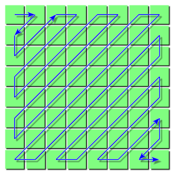
The zigzag is done in quite a clever way; there is simply a 64-element array that maps each natural index to its zigzag order.

// unzig maps from the zig-zag ordering to the natural ordering. For example,
// unzig[3] is the column and row of the fourth element in zig-zag order. The
// value is 16, which means first column (16%8 == 0) and third row (16/8 == 2).
var unzig = [blockSize]int{
	0, 1, 8, 16, 9, 2, 3, 10,
	17, 24, 32, 25, 18, 11, 4, 5,
	12, 19, 26, 33, 40, 48, 41, 34,
	27, 20, 13, 6, 7, 14, 21, 28,
	35, 42, 49, 56, 57, 50, 43, 36,
	29, 22, 15, 23, 30, 37, 44, 51,
	58, 59, 52, 45, 38, 31, 39, 46,
	53, 60, 61, 54, 47, 55, 62, 63,
}

Putting all the pieces together, the JPEG core loop is:

// writeBlock writes a block of pixel data using the given quantization table,
// returning the post-quantized DC value of the DCT-transformed block. b is in
// natural (not zig-zag) order.
func (e *encoder) writeBlock(b *block, q quantIndex, prevDC int32) int32 {
	fdct(b) // apply DCT
	// ...
	for zig := 1; zig < blockSize; zig++ {
		ac := div(b[unzig[zig]], 8*int32(e.quant[q][zig])) // divide zigzag DCT result by quantization number
		if ac == 0 {
			// quantization result is 0, increase RLE
			runLength++
		} else {
			// ...
			// write the current RLE sequence
			e.emitHuffRLE(h, runLength, ac)
			runLength = 0
		}
	}
	//...
}

We’re skipping over quite a bit of detail, but we can see how the different ideas we’ve explored are used.

JPEG is truly a treasure trove of delightful engineering marvels, and what we’ve discussed here is just the appetizer. There’s a lot more to explore, but I hope this has been both enjoyable and informative.

This is it for now. I appreciate you joining me on this journey.

Thank you!